
Ramblings on Math and Programming by Benjamin Kovach
Friday, January 3, 2014
Wednesday, November 13, 2013
Parsing and Negating Boolean Strings in Haskell
It appears that the dailyprogrammer subreddit is back after a pretty long hiatus, and they kicked back into gear with a really interesting problem. The problem was, paraphrasing:
Given a Boolean expression as a string S, compute and print the negation of S as a string using DeMorgan's laws.The problem is also detailed in full here.
I completed the challenge and posted my solution to reddit, but wanted to share it here as well, so here it is, with slight modifications:
This is a problem that is heavily suited to three major things that Haskell advocates: Algebraic Data Types, Pattern Matching, and Monadic Parsing.
First off, if you've had any experience with automata theory, it's pretty clear that the input language of Boolean expressions can be represented by a context free grammar. It just so happens that Haskell makes it incredibly easy to model CFGs right out of the box using Algebraic Data Types. Let's take a look at this data type representing Boolean expressions:
This file contains hidden or bidirectional Unicode text that may be interpreted or compiled differently than what appears below. To review, open the file in an editor that reveals hidden Unicode characters.
Learn more about bidirectional Unicode characters
| data Expr = Not Expr | |
| | And Expr Expr | |
| | Or Expr Expr | |
| | SubExpr Expr | |
| | Var Char | |
| deriving Eq |
Simple. Now, the main problem of this challenge was actually performing the simplification of the not operation. Using pattern matching, we can directly encode these rules in the following manner:
This file contains hidden or bidirectional Unicode text that may be interpreted or compiled differently than what appears below. To review, open the file in an editor that reveals hidden Unicode characters.
Learn more about bidirectional Unicode characters
| not :: Expr -> Expr | |
| not (Not e) = e | |
| not (And e1 e2) = Or (not e1) (not e2) | |
| not (Or e1 e2) = And (not e1) (not e2) | |
| not (SubExpr e) = not e | |
| not (Var c) = Not (Var c) |
Here we're giving a literal definition of rules for negating Boolean expressions. If you use Haskell, this is really easy to read. If you don't: stare at it for a second; you'll see what it's doing! That's the brunt of the challenge, right there. That's it. Encode a Boolean expression into an
Expr and call not on it, and it will spit out a new Expr expressing the negation of your original expression. DeMorgan's laws are represented in the And and Or rules.We can also do this in a slightly modified way, using a function simplify :: Expr -> Expr that simplifies expressions and another function not = simplify . Not. Not to compute the same thing. It's a similar solution so I won't post it, but if you'd like to, feel free to experiment and/or add more simplification rules (e.g. simplify e@(And a b) = if a == b then a else e). We can also display our expressions as a string by declaring Expr an instance of Show in the following way:
This file contains hidden or bidirectional Unicode text that may be interpreted or compiled differently than what appears below. To review, open the file in an editor that reveals hidden Unicode characters.
Learn more about bidirectional Unicode characters
| instance Show Expr where | |
| show (Not e) = "NOT " ++ show e | |
| show (And e1 e2) = show e1 ++ " AND " ++ show e2 | |
| show (Or e1 e2) = show e1 ++ " OR " ++ show e2 | |
| show (Var c) = [c] | |
| show (SubExpr e) = "(" ++ show e ++ ")" |
Now we can type in Boolean expressions using our data type, not them, and print them out as nice expressions. But, now we are faced with, in my opinion, the tougher part of the challenge. We're able to actually compute everything we need to, but what about parsing a Boolean expression (as a string) into an Expr? We can use a monadic parsing library, namely Haskell's beloved Parsec, to do this in a rather simple way. We'll be using Parsec's Token and Expr libraries, as well as the base, in this example. Let's take a look.
This file contains hidden or bidirectional Unicode text that may be interpreted or compiled differently than what appears below. To review, open the file in an editor that reveals hidden Unicode characters.
Learn more about bidirectional Unicode characters
| parseExpr :: String -> Either ParseError Expr | |
| parseExpr = parse expr "" | |
| where expr = buildExpressionParser operators term <?> "compound expression" | |
| term = parens expr <|> variable <?> "full expression" | |
| operators = [ [Prefix (string "NOT" *> spaces *> pure Not)] | |
| , [binary "AND" And] | |
| , [binary "OR" Or] ] | |
| where binary n c = Infix (string n *> spaces *> pure c) AssocLeft | |
| variable = Var <$> (letter <* spaces) <?> "variable" | |
| parens p = SubExpr <$> (char '(' *> spaces *> p <* char ')' <* spaces) <?> "parens" |
We essentially define the structure of our input here and parse it into an Expr using a bunch of case-specific parsing rules.
variable parses a single char into a Var, parens matches and returns a SubExpr, and everything else is handled by using the convenience function buildExpressionParser along with a list of operator strings, the types they translate to and their operator precedence. Here we're using applicative style to do our parsing, but monadic style is fine too. Check this out for more on applicative style parsing.Given that, we can define a main function to read in a file of expressions and output the negation of each of the expressions, like so:
This file contains hidden or bidirectional Unicode text that may be interpreted or compiled differently than what appears below. To review, open the file in an editor that reveals hidden Unicode characters.
Learn more about bidirectional Unicode characters
| main = mapM_ printNotExpr . lines =<< readFile "inputs.txt" | |
| where printNotExpr e = case parseExpr e of | |
| Right x -> print $ not x | |
| Left e -> error $ show e |
Concise and to the point. We make sure that each line gets parsed properly, not the expressions, and print them. Here's what we get when we run the program:
inputs.txt --- outputa --- NOT a
NOT a --- a
a AND b --- NOT a OR NOT b
NOT a AND b --- a OR NOT b
NOT (a AND b) --- a AND b
NOT (a OR b AND c) OR NOT(a AND NOT b) --- (a OR b AND c) AND (a AND NOT b)Thanks for reading.
Tuesday, August 27, 2013
Ludum Dare #27 (10 Seconds): A post-mortem
WTF is Ludum Dare?
Ludum Dare is a friendly competition among game developers to see who can make the best game based on a given theme in 48 hours. This was the 27th competition, and the theme was "10 seconds."
Why did I want to participate?
For a long time, I've been looking at the game development community from the outside with a lens that I feel a lot of people tend to see through. I've always considered game development an extremely intricate and difficult field to enter, and I was scared of trying my hand at it for a long time. I have made small clones of other games (pong, sokoban, etc) and I have enjoyed making those games, but they're both relatively simple (exercise-sized, almost, to a certain extent). I have been wanting to get a little further into the game development scene for a while, and Ludum Dare seemed like the perfect opportunity. I've se
en several Ludum Dare competitions go by over the past couple of years and I never thought I was good enough to actually do it. This time, I just went for it, and I'm really glad I did.
What did you make?
 When the theme "10 seconds" was announced, I had a billion and one ideas going through my head, because it's so open-ended. Everyone's first idea was to make a 10-second game, but that doesn't really work, so you had to move on to the next thing. I bounced a couple of ideas around in my head, but I ultimately decided to make a twin-stick roguelike-like because:
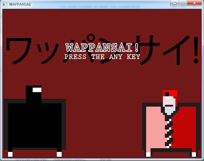
Anyway, in Wappansai!, you're a big fat square ninja man who is stuck in a dungeon with some red business-men enemies. They don't move, but if you don't murder all of the enemies in the room within 10 seconds, you die. Running into enemies also kills you, as does falling into the many pits laid out around the room. Later on, moving spike tiles get added, and those kill you as well. When you clear a room under 10 seconds, a door opens up and you move on to the next room where things get progressively more difficult. I think my high score in the final version of the game was somewhere around 17 rooms, so I definitely challenge everyone to beat that!
Oh, and the tools I used were C++ and SDL 2.0, sfxr for sound bytes, and photoshop for graphics. I didn't get around to making music because I don't even know where to start with that!
What did you learn?
I have been reading Programming Game AI by Example on and off for a little while, and I decided to use Ludum Dare as an opportunity to start learning a little more about the State Design Pattern and Singletons, two concepts introduced early on in that book. I worked on throwing together a shell of a program that implemented these things before the competition, so I wouldn't have to figure everything out as I was trying to get things done over the 48 hours, which was definitely a good idea. I was able to start working right when the clock started ticking instead of worrying about getting the design right as I was trying to implement the program. I'd recommend doing this if you plan to participate in a game jam; it really helped me out. That said, there were still some design pitfalls. For example, when you open chests in the game, there's a (very slim) chance that you'll get a laser gun from inside of it (usually it just takes all of your currently held items -- haha!), but the gun doesn't spawn anywhere when this happens; it just magically goes into your character's weapon slot and suddenly you're firing lasers. The way I wanted this to work was, if you got lucky and got the laser gun from the chest, the gun would spawn somewhere on the map and you could go pick it up and feel awesome that that chest that normally screws you over by stealing all of your items just happened to spawn a freakin' laser gun for you to play with. But, the way I organized my project, Tile objects had no way to modify Level objects, so I was unable to trigger an event when the chest (a type of Tile) was touched to modify the level (a Level), so I had to make a compromise there. There are certainly workarounds that I considered, but I couldn't really do them within the time limit. It was a design flaw, and now I know that it was a design flaw. I can structure my code better now -- that was one major learning point.
I also learned a lot about randomly generated content, that was crazy! It actually went a lot smoother than I thought it would, but just seeing everything so randomized was amazing. Items, weapons, enemies, pits, and walls all get generated randomly based on how many rooms you've traversed, and just seeing that in play working (relatively) nicely was so cool. So I learned a lot there.
The final, really huge thing that I discovered was that...holy crap, there are a lot of assets that go into games! I must have made over 50 sprites for Wappansai!, on top of tons of different sound clips (sfxr made this easy). A lot more time went into art than I expected, and I didn't even animate anything...you don't really think about it, but games have tons and tons of assets involved.
Would I do it again?
Finishing a game in two days was really hard work and it could be really frustrating at times (especially using C++ with VS, those error messages are completely incomprehensible). But, it was totally worth the effort. I can say that I've made a game that is completely mine, and even though it's not very good, it's something that I made and I love that I made it and I'm excited to make more things. It's also really amazing that people actually do play your games. I've had several comments on my ludum dare game's page already discussing the game that I made, and it's so cool to see that. Playing everyone else's games is also really awesome because you know that they went through the same thing that you did. Everyone's really proud of their work, everyone worked hard to get something done, and it's just a really nice community event that I'm so happy to have been a part of. I would absolutely do it again, and plan to!
Who would I recommend Ludum Dare to?
If you want to make games, do it. If you don't know where to start, there are plenty of websites that can teach you the basics, and even if you don't want/ know how to program, there are tools out there like GameMaker Studio that will allow you to program your game's logic without actually writing code. If you don't think you can do it alone, team up with someone. But if you want to make video games and have at least a basic knowledge of how they work, I think that Ludum Dare is an excellent way to test your skills and build something that you'll be proud of.
Where can I download your game?
You can download, rate, and comment on Wappansai! over at the Ludum Dare page for it.
Thanks for reading!
5outh
Ludum Dare is a friendly competition among game developers to see who can make the best game based on a given theme in 48 hours. This was the 27th competition, and the theme was "10 seconds."
Why did I want to participate?
For a long time, I've been looking at the game development community from the outside with a lens that I feel a lot of people tend to see through. I've always considered game development an extremely intricate and difficult field to enter, and I was scared of trying my hand at it for a long time. I have made small clones of other games (pong, sokoban, etc) and I have enjoyed making those games, but they're both relatively simple (exercise-sized, almost, to a certain extent). I have been wanting to get a little further into the game development scene for a while, and Ludum Dare seemed like the perfect opportunity. I've se
en several Ludum Dare competitions go by over the past couple of years and I never thought I was good enough to actually do it. This time, I just went for it, and I'm really glad I did.
 When the theme "10 seconds" was announced, I had a billion and one ideas going through my head, because it's so open-ended. Everyone's first idea was to make a 10-second game, but that doesn't really work, so you had to move on to the next thing. I bounced a couple of ideas around in my head, but I ultimately decided to make a twin-stick roguelike-like because:
- Movement and collision detection is relatively simple to implement, and
- As all of my friends know, I'm a big fan of The Binding of Isaac, and I'm always thinking about how that game and games similar in nature to it are put together.
Anyway, in Wappansai!, you're a big fat square ninja man who is stuck in a dungeon with some red business-men enemies. They don't move, but if you don't murder all of the enemies in the room within 10 seconds, you die. Running into enemies also kills you, as does falling into the many pits laid out around the room. Later on, moving spike tiles get added, and those kill you as well. When you clear a room under 10 seconds, a door opens up and you move on to the next room where things get progressively more difficult. I think my high score in the final version of the game was somewhere around 17 rooms, so I definitely challenge everyone to beat that!
Oh, and the tools I used were C++ and SDL 2.0, sfxr for sound bytes, and photoshop for graphics. I didn't get around to making music because I don't even know where to start with that!
What did you learn?
I have been reading Programming Game AI by Example on and off for a little while, and I decided to use Ludum Dare as an opportunity to start learning a little more about the State Design Pattern and Singletons, two concepts introduced early on in that book. I worked on throwing together a shell of a program that implemented these things before the competition, so I wouldn't have to figure everything out as I was trying to get things done over the 48 hours, which was definitely a good idea. I was able to start working right when the clock started ticking instead of worrying about getting the design right as I was trying to implement the program. I'd recommend doing this if you plan to participate in a game jam; it really helped me out. That said, there were still some design pitfalls. For example, when you open chests in the game, there's a (very slim) chance that you'll get a laser gun from inside of it (usually it just takes all of your currently held items -- haha!), but the gun doesn't spawn anywhere when this happens; it just magically goes into your character's weapon slot and suddenly you're firing lasers. The way I wanted this to work was, if you got lucky and got the laser gun from the chest, the gun would spawn somewhere on the map and you could go pick it up and feel awesome that that chest that normally screws you over by stealing all of your items just happened to spawn a freakin' laser gun for you to play with. But, the way I organized my project, Tile objects had no way to modify Level objects, so I was unable to trigger an event when the chest (a type of Tile) was touched to modify the level (a Level), so I had to make a compromise there. There are certainly workarounds that I considered, but I couldn't really do them within the time limit. It was a design flaw, and now I know that it was a design flaw. I can structure my code better now -- that was one major learning point.
 |
| Randomly Generated...everything! |
The final, really huge thing that I discovered was that...holy crap, there are a lot of assets that go into games! I must have made over 50 sprites for Wappansai!, on top of tons of different sound clips (sfxr made this easy). A lot more time went into art than I expected, and I didn't even animate anything...you don't really think about it, but games have tons and tons of assets involved.
Would I do it again?
Finishing a game in two days was really hard work and it could be really frustrating at times (especially using C++ with VS, those error messages are completely incomprehensible). But, it was totally worth the effort. I can say that I've made a game that is completely mine, and even though it's not very good, it's something that I made and I love that I made it and I'm excited to make more things. It's also really amazing that people actually do play your games. I've had several comments on my ludum dare game's page already discussing the game that I made, and it's so cool to see that. Playing everyone else's games is also really awesome because you know that they went through the same thing that you did. Everyone's really proud of their work, everyone worked hard to get something done, and it's just a really nice community event that I'm so happy to have been a part of. I would absolutely do it again, and plan to!
Who would I recommend Ludum Dare to?
 |
| As you can see, my game had Dark Souls elements. |
Where can I download your game?
You can download, rate, and comment on Wappansai! over at the Ludum Dare page for it.
Thanks for reading!
5outh
Wednesday, May 1, 2013
Symbolic Calculus in Haskell
Motivation
It's relatively simple to write a program to approximate derivatives. We simply look at the limit definition of a derivative:\frac{d}{dx} f(x) = \lim_{h \rightarrow 0} \frac{f(x+h) - f(x)}{h}
and choose some small decimal number to use for h instead of calculating the limit of the function as it goes to 0. Generally, this works pretty well. We get good approximations as long as h is small enough. However, these approximations are not quite exact, and they can only be evaluated at specific points (for example, we can find \frac{d}{dx}f(5), but not the actual symbolic function). So, what if we want to know what \frac{d}{dx}f(x) is for all x? Calculating derivatives with this approximation method won't do the trick for us -- we'll need something a little more powerful, which is what we will build in this post.
Admittedly, this idea didn't come to me through necessity of such a system; I was just curious. It ended up being pretty enlightening, and it's amazing how simple Haskell makes this type of thing. Most of the code in this post didn't take too long to write, it's relatively short (only 108 lines total, including whitespace) and has a lot of capability.
With that, let's get started!
The Data Type
I don't want to over-complicate the process of taking derivatives, so my data type for algebraic expressions is kept minimal.
We support six different types of expressions:
We support six different types of expressions:
- Variables (denoted by a single character)
- Constant values
- Addition
- Multiplication
- Exponentiation
- Division
This can be expanded upon, but this is adequate for the purpose of demonstration.
Here is our Expr a type, with a sample expression representing 3x^2:
This file contains hidden or bidirectional Unicode text that may be interpreted or compiled differently than what appears below. To review, open the file in an editor that reveals hidden Unicode characters.
Learn more about bidirectional Unicode characters
| infixl 4 :+: | |
| infixl 5 :*:, :/: | |
| infixr 6 :^: | |
| data Expr a = Var Char | |
| | Const a | |
| | (Expr a) :+: (Expr a) | |
| | (Expr a) :*: (Expr a) | |
| | (Expr a) :^: (Expr a) | |
| | (Expr a) :/: (Expr a) | |
| deriving (Show, Eq) | |
| sampleExpr :: Expr Double | |
| sampleExpr = Const 3 :*: Var 'x' :^: Const 2 --3x^2 |
Haskell allows infix operators to act as data constructors, which allows us to express algebraic expressions cleanly and concisely without too much mental parsing. Also note that, since we explicitly defined operator precedence above the data type declaration, we can write expressions without parentheses according to order of operations, like we did in the sample expression.
The Algebra
Taking derivatives simply by the rules can get messy, so we might as well go ahead and set up an algebra simplification function that cleans up our final expressions for us. This is actually incredibly simple. As long as you know algebraic laws, this kind of thing basically writes itself in Haskell. We just need to pattern match against certain expressions and meld them together according to algebraic law.This function ends up being lengthy long due to the fact that symbolic manipulation is mostly just a bunch of different cases, but we can encode algebraic simplification rules for our above data type in a straightforward way.
The following simplify function takes an expression and spits out a simpler one that means the same thing. It's really just a bunch of pattern-matching cases, so feel free to skim it.
This file contains hidden or bidirectional Unicode text that may be interpreted or compiled differently than what appears below. To review, open the file in an editor that reveals hidden Unicode characters.
Learn more about bidirectional Unicode characters
| simplify :: (Num a, Eq a, Floating a) => Expr a -> Expr a | |
| simplify (Const a :+: Const b) = Const (a + b) | |
| simplify (a :+: Const 0) = simplify a | |
| simplify (Const 0 :+: a ) = simplify a | |
| simplify (Const a :*: Const b) = Const (a*b) | |
| simplify (a :*: Const 1) = simplify a | |
| simplify (Const 1 :*: a) = simplify a | |
| simplify (a :*: Const 0) = Const 0 | |
| simplify (Const 0 :*: a) = Const 0 | |
| simplify (Const a :^: Const b) = Const (a**b) | |
| simplify (a :^: Const 1) = simplify a | |
| simplify (a :^: Const 0) = Const 1 | |
| simplify ((c :^: Const b) :^: Const a) = c :^: (Const (a*b)) | |
| simplify (Const a :*: (Const b :*: expr)) = (Const $ a*b) :*: (simplify expr) | |
| simplify (Const a :*: expr :*: Const b) = (Const $ a*b) :*: (simplify expr) | |
| simplify (expr :*: Const a :*: Const b) = (Const $ a*b) :*: (simplify expr) | |
| simplify (Const a :*: (b :+: c)) = (Const a :*: (simplify b)) :+: (Const a :*: (simplify c)) | |
| simplify (Const 0 :/: a ) = Const 0 | |
| simplify (Const a :/: Const 0) = error "Division by zero!" | |
| simplify (Const a :/: Const b) | a == b = Const 1 -- only when a == b | |
| simplify (a :/: Const 1) = simplify a | |
| simplify (a :/: b) = (simplify a) :/: (simplify b) | |
| simplify (a :^: b) = (simplify a) :^: (simplify b) | |
| simplify (a :*: b) = (simplify a) :*: (simplify b) | |
| simplify (a :+: b) = (simplify a) :+: (simplify b) | |
| simplify x = id x | |
| fullSimplify expr = fullSimplify' expr (Const 0) -- placeholder | |
| where fullSimplify' cur last | cur == last = cur | |
| | otherwise = let cur' = simplify cur | |
| in fullSimplify' cur' cur |
I've also included a fullSimplify function that runs simplify on an expression until the current input matches the last output of simplify (which ensures an expression is completely simplified)*. Note that in the simplify function, I've covered a lot of bases, but not all of them. Specifically, division simplification is lacking because it gets complicated quickly and I didn't want to focus on that in this blog post.
We should also note that we don't have a data type expressing subtraction or negative numbers, so we'll deal with that now. In order to express the negation of expressions, we define the negate' function, which basically multiplies expressions by -1 and outputs the resultant expression.
This file contains hidden or bidirectional Unicode text that may be interpreted or compiled differently than what appears below. To review, open the file in an editor that reveals hidden Unicode characters.
Learn more about bidirectional Unicode characters
| negate' :: (Num a) => Expr a -> Expr a | |
| negate' (Var c) = (Const (-1)) :*: (Var c) | |
| negate' (Const a) = Const (-a) | |
| negate' (a :+: b) = (negate' a) :+: (negate' b) | |
| negate' (a :*: b) = (negate' a) :*: b | |
| negate' (a :^: b) = Const (-1) :*: a :^: b | |
| negate' (a :/: b) = (negate' a) :/: b |
Now we have a relatively robust system for computing symbolic expressions. However, we aren't able to actually plug anything into these expressions yet, so we'll fix that now.
*Thanks to zoells on Reddit for the suggestion!
Evaluating Expressions
The first thing we'll need to do to begin the process of evaluating expressions is write a function to plug in a value for a specific variable. We do this in terms of a function called mapVar, implemented as follows:
This file contains hidden or bidirectional Unicode text that may be interpreted or compiled differently than what appears below. To review, open the file in an editor that reveals hidden Unicode characters.
Learn more about bidirectional Unicode characters
| mapVar :: (Char -> Expr a) => Expr a -> Expr a | |
| mapVar f (Var d) = f d | |
| mapVar _ (Const a) = Const a | |
| mapVar f (a :+: b) = (mapVar f a) :+: (mapVar f b) | |
| mapVar f (a :*: b) = (mapVar f a) :*: (mapVar f b) | |
| mapVar f (a :^: b) = (mapVar f a) :^: (mapVar f b) | |
| mapVar f (a :/: b) = (mapVar f a) :/: (mapVar f b) | |
| plugIn :: Char -> a -> Expr a -> Expr a | |
| plugIn c val = mapVar (\x -> if x == c then Const val else Var x) |
mapVar searches through an expression for a specific variable and performs a function on each instance of that variable in the function. plugIn takes a character and a value, and is defined using mapVar to map variables with a specific name to a constant provided by the user.
Now that we have plugIn, we can define two functions: One that takes an expression full of only constants and outputs a result (evalExpr'), and one that will replace a single variable with a constant and output the result (evalExpr):
This file contains hidden or bidirectional Unicode text that may be interpreted or compiled differently than what appears below. To review, open the file in an editor that reveals hidden Unicode characters.
Learn more about bidirectional Unicode characters
| evalExpr :: (Num a, Floating a) => Char -> a -> Expr a -> a | |
| evalExpr c x = evalExpr' . plugIn c x | |
| evalExpr' :: (Num a, Floating a) => Expr a -> a | |
| evalExpr' (Const a) = a | |
| evalExpr' (Var c) = error $ "Variables (" | |
| ++ [c] ++ | |
| ") still exist in formula. Try plugging in a value!" | |
| evalExpr' (a :+: b) = (evalExpr' a) + (evalExpr' b) | |
| evalExpr' (a :*: b) = (evalExpr' a) * (evalExpr' b) | |
| evalExpr' (a :^: b) = (evalExpr' a) ** (evalExpr' b) | |
| evalExpr' (a :/: b) = (evalExpr' a) / (evalExpr' b) |
What we're doing here is simple. With evalExpr', we only need to replace our functional types (:+:, :*:, etc) with the actual functions (+, *, etc). When we run into a Const, we simply replace it with it's inner number value. When we run into a Var, we note that it's not possible to evaluate, and tell the user that there is still a variable in the expression that needs to be plugged in.
With evalExpr, we just plug in a value for a specific variable before evaluating the expression. Simple as that!
Here are some examples of expressions and their evaluations:
*Main> evalExpr 'x' 2 (Var 'x')
2.0
*Main> evalExpr 'a' 3 (Const 3 :+: Var 'a' :*: Const 6)
21.0
*Main> evalExpr 'b' 2 (Var 'b' :/: (Const 2 :*: Var 'b'))
0.5
We can even evaluate multivariate expressions using plugIn:
*Main> evalExpr' . plugIn 'x' 1 $ plugIn 'y' 2 (Var 'x' :+: Var 'y')
3.0
Now that we've extended our symbolic expressions to be able to be evaluated, let's do what we set out to do -- find derivatives!
Derivatives
We aren't going to get into super-complicated derivatives involving logorithmic or implicit differentiation, etc. Instead, we'll keep it simple for now, and only adhere to some of the 'simple' derivative rules. We'll need one of them for each of our six expression types: constants, variables, addition, multiplication, division, and exponentiation. We already know the following laws for these from calculus:Differentiation of a constant: \frac{d}{dx}k = 0
Differentiation of a variable: \frac{d}{dx}x = 1
Addition differentiation: \frac{d}{dx}\left(f(x) + g(x)\right) = \frac{d}{dx}f(x) +\frac{d}{dx}g(x)
Power rule (/chain rule): \frac{d}{dx}f(x)^n = nf(x)^{n-1} \cdot \frac{d}{dx}f(x)
Product rule: \frac{d}{dx}\left(f(x) \cdot g(x)\right) = \frac{d}{dx}f(x) \cdot g(x) + f(x) \cdot \frac{d}{dx}g(x)
Quotient rule: \frac{d}{dx}\frac{f(x)}{g(x)} = \frac{\frac{d}{dx}f(x) \cdot g(x) - \frac{d}{dx}g(x) \cdot f(x)}{g(x)^2}
As it turns out, we can almost directly represent this in Haskell. There should be no surprises here -- following along with the above rules, it is relatively easy to see how this function calculates derivatives. We will still error out if we get something like x^x as input, as it will require a technique we haven't implemented yet. However, this will suffice for a many different expressions.
This file contains hidden or bidirectional Unicode text that may be interpreted or compiled differently than what appears below. To review, open the file in an editor that reveals hidden Unicode characters.
Learn more about bidirectional Unicode characters
| derivative :: (Num a) => Expr a -> Expr a | |
| derivative (Var c) = Const 1 | |
| derivative (Const x) = Const 0 | |
| --product rule (ab' + a'b) | |
| derivative (a :*: b) = (a :*: (derivative b)) :+: (b :*: (derivative a)) -- product rule | |
| --power rule (xa^(x-1) * a') | |
| derivative (a :^: (Const x)) = ((Const x) :*: (a :^: (Const $ x-1))) :*: (derivative a) | |
| derivative (a :+: b) = (derivative a) :+: (derivative b) | |
| -- quotient rule ( (a'b - b'a) / b^2 ) | |
| derivative (a :/: b) = ((derivative a :*: b) :+: (negate' (derivative b :*: a))) | |
| :/: | |
| (b :^: (Const 2)) | |
| derivative expr = error "I'm not a part of your system!" -- unsupported operation |
So, what can we do with this? Well, let's take a look:
This file contains hidden or bidirectional Unicode text that may be interpreted or compiled differently than what appears below. To review, open the file in an editor that reveals hidden Unicode characters.
Learn more about bidirectional Unicode characters
| ddx :: (Floating a, Eq a) => Expr a -> Expr a | |
| ddx = fullSimplify . derivative | |
| ddxs :: (Floating a, Eq a) => Expr a -> [Expr a] | |
| ddxs = iterate ddx | |
| nthDerivative :: (Floating a, Eq a) => Int -> Expr a -> Expr a | |
| nthDerivative n = foldr1 (.) (replicate n ddx) |
The first, most obvious thing we'll note when running the derivative function on an expression is that what it produces is rather ugly. To fix this, we'll write a function ddx that will simplify the derivative expression three times to make our output cleaner.
(Remember sampleExpr = 3x^2)
*Main> derivative sampleExpr
Const 3.0 :*: ((Const 2.0 :*: Var 'x' :^: Const 1.0) :*: Const 1.0) :+: Var 'x' :^: Const 2.0 :*: Const 0.0
*Main> ddx sampleExpr
Const 6.0 :*: Var 'x' -- 6x
Another thing we can do is get a list of derivatives. The iterate method from the Prelude suits this type of thing perfectly -- we can generate a (infinite!) list of derivatives of a function just by calling iterate ddx. Simple, expressive, and incredibly powerful.
*Main> take 3 $ ddxs sampleExpr
[Const 3.0 :*: Var 'x' :^: Const 2.0,Const 6.0 :*: Var 'x',Const 6.0] -- [3x^2, 6x, 6]
*Main> let ds = take 4 $ ddxs sampleExpr
*Main> fmap (evalExpr 'x' 2) ds
[12.0,12.0,6.0,0.0]
We're also able to grab the n^{th} derivative of an expression. We could simply grab the n^{th} term of ddxs, but we'll do it without the wasted memory by repeatedly composing ddx n times using foldr1 and replicate.
*Main> nthDerivative 2 sampleExpr
Const 6.0
There's one last thing I want to touch on. Since it's so simple to generate a list of derivatives of a function, why not use that to build functions' Taylor series expansions?
Taylor Series Expansions
The Taylor series expansion of a function f(x) about a is defined as follows:\sum_{n=1}^{\infty} \frac{f^{(n)}(a)}{n!} \cdot (x - a)^n
The Maclaurin series expansion for a function is the Taylor series of a function with a = 0, and we will also implement that.
Given that we can:
- Have multivariate expressions
- Easily generate a list of derivatives
We can actually find the Taylor series expansion of a function easily. Again, we can almost directly implement this function in Haskell, and evaluating it is no more difficult.
This file contains hidden or bidirectional Unicode text that may be interpreted or compiled differently than what appears below. To review, open the file in an editor that reveals hidden Unicode characters.
Learn more about bidirectional Unicode characters
| taylor :: (Floating a, Eq a) => Expr a -> [Expr a] | |
| taylor expr = fmap fullSimplify (fmap series exprs) | |
| where indices = fmap fromIntegral [1..] | |
| derivs = fmap (changeVars 'a') (ddxs expr) | |
| where changeVars c = mapVar (\_ -> Var c) | |
| facts = fmap Const $ scanl1 (*) indices | |
| exprs = zip (zipWith (:/:) derivs facts) indices -- f^(n)(a)/n! | |
| series (expr, n) = | |
| expr :*: ((Var 'x' :+: (negate' $ Var 'a')) :^: Const n) -- f^(n)(a)/n! * (x - a)^n | |
| maclaurin = fmap (fullSimplify . plugIn 'a' 0) . taylor | |
| evalTaylorWithPrecision a x prec = | |
| sum . map (evalExpr' . plugIn 'x' x . plugIn 'a' a) . take prec . taylor | |
| evalTaylor a x = evalTaylorWithPrecision a x 100 | |
| evalMaclaurin = evalTaylor 0 | |
| evalMacLaurinWithPrecision = evalTaylorWithPrecision 0 |
To produce a Taylor series, we need a couple of things:
- A list of derivatives
- A list of indices
- A list of factorials
We create these three things in where clauses in the taylor declaration. indices are simple, derivs calculates a list of derivatives (using mapVar again to change all variables into as), and facts contains our factorials wrapped in Consts. We generate a list of (expression, index)s in exprs, and then map the "gluing" function series over exprs to produce a list of expressions in the series expansion. We then fmap superSimplify over the list in order to simplify down our expressions, and we get back a list of Taylor series terms for the given expression. The Maclaurin expansion can be defined as mentioned above in terms of the Taylor series, and again, we basically directly encode it (though we do have to re-simplify our expressions due to the plugging in of a variable).
Let's take a look at the Taylor expansion for f(x) = x. We note that:
f(a) = a
f'(a) = 1
f''(a) = 0
And the rest of the derivatives will be 0. So our Taylor series terms T_n should look something like:
T_1 = \frac{a}{1} \cdot (x - a) = a \cdot (x-a)
T_2 = \frac{1}{2} \cdot (x-a)^2
T_3 = \frac{0}{6} \cdot (x-a)^3 = 0
...and so on. Let's take a look at what taylor produces:
*Main> take 3 $ taylor (Var 'x')
[Var 'a' :*: (Var 'x' :+: Const (-1.0) :*: Var 'a'),
--^ a * (x-a)
(Const 1.0 :/: Const 2.0) :*: (Var 'x' :+: Const (-1.0) :*: Var 'a') :^: Const 2.0,
--^ 1/2 * (x-a)^2
Const 0.0]
This matches what we determined earlier.
To evaluate a Taylor expression, we need a value for a, a value for x, and a specified number of terms for precision. We default this precision to 100 terms in the evalTaylor function, and the logic takes place in the evalTaylorWithPrecision function. In this function, we get the Taylor expansion, take the first prec terms, plug in a and x for all values of the function, and finally sum the terms. Maclaurin evaluation is again defined in terms of Taylor evaluation.
Taking a look at the above Taylor series expansion of f(x) = x, there is only one term where a zero-valued a will produce any output (namely \frac{1}{2} \cdot (x-a)^2). So when we evaluate our Maclaurin series for this function at x, we should simply get back \frac{1}{2}x^2. Let's see how it works:
*Main> evalMaclaurin 2 (Var 'x')
2.0 --1/2 2^2 = 1/2 * 4 = 2
*Main> evalMaclaurin 3 (Var 'x')
4.5 -- 1/2 * 3^2 = 1/2 * 9 = 4.5
*Main> evalMaclaurin 10 (Var 'x')
50.0 -- 1/2 * 10^2 = 1/2 * 100 = 50
Looks like everything's working!
Please leave any questions, suggestions, etc, in the comments!
Until next time,
Ben
Thursday, January 24, 2013
Graph Theory and the Handshake Problem
The Handshake Problem
The Handshake Problem is something of a classic in mathematics. I first heard about it in an algebra course I took in high school, and it's stuck with me through the years. The question is this:
In a room containing n people, how many handshakes must take place for everyone to have shaken hands with everyone else?The goal of this short blog post will be to present a solution to this problem using the concept of graphs.
The Complete Graph
 |
| fig. I: A complete graph with 7 vertices |
We can use the model of a complete graph to reason about the problem at hand. The nodes in the graph may represent the people in the room, while the connecting edges represent the handshakes that must take place. As such, the key to solving the Handshake Problem is to count the edges in a complete graph.
But it would be silly to draw out a graph and count the edges one-by-one in order to solve this problem (and would take a very long time for large values of n), so we'll use math!
The Solution
To find the solution, we have to make a few key observations. The easiest way to start out in this case is to map out the first few complete graphs and try to find a pattern:
Let n = the number of nodes, e = the number of edges.
- n = 1 \Rightarrow e = 0
- n = 2 \Rightarrow e = 1
- n = 3 \Rightarrow e = 3
- n = 4 \Rightarrow e = 6
It follows that the number of the edges (e) in a complete graph with n vertices can be represented by the sum (n-1) + (n-2) + \dots + 1 + 0, or more compactly as:
\sum_{i=1}^n i-1
You may already know from summation laws that this evaluates to \frac{n(n-1)}{2}. Let's prove it.
The Proof
Theorem: \forall n \in \mathbb{N} : \sum_{i=1}^{n} i-1 = \frac{n(n-1)}{2}
Proof: Base case: Let n = 1. Then, \frac{1(1-1)}{2} = \sum_{i=1}^1 i-1 = 0.
Inductive case: Let n \in \mathbb{N}. We need to prove that \frac{n(n-1)}{2} + n = \frac{n(n+1)}{2}.
\begin{array} {lcl} \frac{n(n-1)}{2} + n & = & \frac{n(n-1)+2n}{2} \\ & = & \frac{n^2 - n + 2n}{2} \\ & = & \frac{n^2 + n}{2} \\ & = & \frac{n(n+1)}{2}■\end{array}
We can now use the theorem knowing it's correct, and, in fact, provide a solution to the original problem. The answer to the Handshake Problem involving n people in a room is simply \frac{n(n-1)}{2}. So, the next time someone asks you how many handshakes would have to take place in order for everyone in a room with 1029 people to shake each other's hands, you can proudly answer "528906 handshakes!"
Until next time,
Ben
Wednesday, January 16, 2013
Comonadic Trees
We've seen in the previous post what monads are and how they work. We saw a few monad instances of some common Haskell structures and toyed around with them a little bit. Towards the end of the post, I asked about making a Monad instance for a generalized tree data type. My guess is that it was relatively difficult. But why?
Well, one thing that I didn't touch on in my last post was that the monadic >>= operation can also be represented as (join . fmap f), that is, a >>= f = join \$ fmap f a, as long as a has a Functor instance.
join is a generalized function of the following type:
join :: (Monad ~m) \Rightarrow m ~(m ~a) \rightarrow m ~a
Basically, this function takes a nested monad and "joins" it with the top level in order to get a regular m a out of it. Since you bind to functions that take as and produce m as, fmap f actually makes m (m a)s and join is just the tool to fix up the >>= function to produce what we want.
Keep in mind that join is not a part of the Monad typeclass, and therefore the above definition for >>= will not work. However, if we are able to make a specific join function (named something else, since join is taken!) for whatever type we are making a Monad instance for, we can certainly use the above definition.
I don't want to spend too much time on this, but I would like to direct the reader to the Monad instance for [] that I mentioned in the last post -- can you see any similarities between this and the way I structured >>= above?
Now back to the Tree type. Can you devise some way to join Trees? That is, can you think of a way to flatten a Tree of Tree as into a Tree a?
This actually turns out to be quite difficult, and up to interpretation as to how you want to do it. It's not as straightforward as moving Maybe (Maybe a)s into Maybe as or [[a]]s into [a]s. Maybe if we put a Monoid restriction on our a type, as such...
instance ~(Monoid ~a) \Rightarrow Monad ~(Tree ~a) ~where ~\dots
...we could use mappend in some way in order to concatenate all of the nested elements using some joining function. While this is a valid way to define a Tree Monad, it seems a little bit "unnatural." I won't delve too deeply into that, though, because that's not the point of this post. Let's instead take a look at a structure related to monads that may make more sense for our generalized Tree type.
(>>=) :: (Monad ~m) \Rightarrow m ~a \rightarrow ~(a \rightarrow m ~b) \rightarrow m ~b
That is, we're taking an m a and converting it to an m b by means of some function that operates on the contained type. In other words, we're producing a new value using elements contained inside the Monad. Comonads have a similar function:
(=>>) :: (Comonad ~w) \Rightarrow w ~a \rightarrow (w ~a \rightarrow ~b) \rightarrow w ~b
The difference here is that the function that we use to produce a new value operates on the whole -- we're not operating on the elements contained inside the Comonad, but the Comonad itself, to produce a new value.
We also have a function similar to the Monadic return:
coreturn :: (Comonad ~w) \Rightarrow w ~a \rightarrow a
Whereas return puts a value into a Monadic context, coreturn extracts a value from a Comonadic context.
I mentioned the Monadic join function above because I would also like to mention that there is a similar operation for Comonads:
cojoin :: (Comonad ~w) \Rightarrow w ~a \rightarrow w ~(w ~a)
Instead of "removing a layer," we're "adding" a layer. And, as it turns out, just as a >>= f can be represented as join \$ fmap f a, =>> can be represented as:
a ~=>> ~f = fmap ~f ~\$ ~cojoin ~a
The full Comonad typeclass (as I like to define it) is as follows:
class ~(Functor ~w) \Rightarrow Comonad ~w ~a ~where \\ \hspace{22pt}coreturn :: (Comonad ~w) \Rightarrow w ~a \rightarrow a \\ \hspace{38pt}cojoin :: (Comonad ~w) \Rightarrow w ~a \rightarrow w ~(w ~a) \\ a ~=>> ~f = fmap ~f ~\$ ~cojoin ~a
By now, it should at least be clear that Monads and Comonads are related -- it shouldn't be hard to see why they are so similar in name!
Note: There is a package called Control.Comonad on Hackage. It uses different names for the Comonad operations, but they do the same things. It's a good package, but I wanted to show how Comonads are built and use the operation names I used to make things clearer.
As it turns out, the Tree a structure that I've been mentioning fits into the Comonadic context quite well, and provides a simple example as to how Comonads work.
Then we'll go ahead and make a Functor instance of our Tree a data type:
From here, we're able to make a Comonadic Tree like so:
The only real point of confusion here is in the cojoin function for Nodes. But, all we are doing is wrapping the entire node in a new node, and then mapping cojoin over every child node of the current node to produce its children. In other words, we're turning a Node a into a Node (Node a), which is exactly what we want to do.
So what can we do with a comonadic tree? Let's tackle a simple problem. Say we're hanging out in California, and we want to get to the East coast as quickly as possible. We don't really care where on the East coast we end up -- we just want to get there. We can map out the different paths that we can take, along with the time it takes to get to each one. In other words, we're going to model spots on the map as Nodes on a Tree and give them a weight corresponding to the time it takes to get there. We can model this situation with a Tree as follows:
The number of each Node marks its distance from the previous Node. The root Node of the Tree is the starting point, so it is 0 distance away from itself.
What we want to do to find the shortest path through the country is essentially, as follows. First, we're going to need to check the deepest nodes, and find their minimum distance children. We will add the distance of the Node closest to the one we're examining to its own distance, to find the shortest way to get from the node we're examining to the destination. Once all of that has been done, we'll need to traverse up the tree, repeating this as we go. By the end of the algorithm, the root Node will be marked with the shortest distance to the destination.
Now, that may sound somewhat iterative in nature, but we're going to morph this into a comonadic operation. First, let's take a look at a function we can use to find the minimum distance to the next level of our tree:
This is relatively simple, and does precisely what was mentioned above: adds the minimum value contained in the connected Nodes to the parent Node. Next, take a look at the type signature. We can see that this function produces a new number from a tree full of numbers. This coincides precisely with the function type we need to use with =>>, so we'll be able to use it to get exactly what we want.
The rest is very simple:
This produces a tree full of the minimum distances from each node to the East coast. Pulling the actual value out is as easy as calling coreturn on the resultant tree.
Thanks for reading!
Ben
For further reading on Comonads, I recommend the article Evaluating Cellular Automata is Comonadic.
Well, one thing that I didn't touch on in my last post was that the monadic >>= operation can also be represented as (join . fmap f), that is, a >>= f = join \$ fmap f a, as long as a has a Functor instance.
join is a generalized function of the following type:
join :: (Monad ~m) \Rightarrow m ~(m ~a) \rightarrow m ~a
Basically, this function takes a nested monad and "joins" it with the top level in order to get a regular m a out of it. Since you bind to functions that take as and produce m as, fmap f actually makes m (m a)s and join is just the tool to fix up the >>= function to produce what we want.
Keep in mind that join is not a part of the Monad typeclass, and therefore the above definition for >>= will not work. However, if we are able to make a specific join function (named something else, since join is taken!) for whatever type we are making a Monad instance for, we can certainly use the above definition.
I don't want to spend too much time on this, but I would like to direct the reader to the Monad instance for [] that I mentioned in the last post -- can you see any similarities between this and the way I structured >>= above?
Now back to the Tree type. Can you devise some way to join Trees? That is, can you think of a way to flatten a Tree of Tree as into a Tree a?
This actually turns out to be quite difficult, and up to interpretation as to how you want to do it. It's not as straightforward as moving Maybe (Maybe a)s into Maybe as or [[a]]s into [a]s. Maybe if we put a Monoid restriction on our a type, as such...
instance ~(Monoid ~a) \Rightarrow Monad ~(Tree ~a) ~where ~\dots
...we could use mappend in some way in order to concatenate all of the nested elements using some joining function. While this is a valid way to define a Tree Monad, it seems a little bit "unnatural." I won't delve too deeply into that, though, because that's not the point of this post. Let's instead take a look at a structure related to monads that may make more sense for our generalized Tree type.
What is a comonad?
Recall the type signature of >>= for Monads:(>>=) :: (Monad ~m) \Rightarrow m ~a \rightarrow ~(a \rightarrow m ~b) \rightarrow m ~b
That is, we're taking an m a and converting it to an m b by means of some function that operates on the contained type. In other words, we're producing a new value using elements contained inside the Monad. Comonads have a similar function:
(=>>) :: (Comonad ~w) \Rightarrow w ~a \rightarrow (w ~a \rightarrow ~b) \rightarrow w ~b
The difference here is that the function that we use to produce a new value operates on the whole -- we're not operating on the elements contained inside the Comonad, but the Comonad itself, to produce a new value.
We also have a function similar to the Monadic return:
coreturn :: (Comonad ~w) \Rightarrow w ~a \rightarrow a
Whereas return puts a value into a Monadic context, coreturn extracts a value from a Comonadic context.
I mentioned the Monadic join function above because I would also like to mention that there is a similar operation for Comonads:
cojoin :: (Comonad ~w) \Rightarrow w ~a \rightarrow w ~(w ~a)
Instead of "removing a layer," we're "adding" a layer. And, as it turns out, just as a >>= f can be represented as join \$ fmap f a, =>> can be represented as:
a ~=>> ~f = fmap ~f ~\$ ~cojoin ~a
The full Comonad typeclass (as I like to define it) is as follows:
class ~(Functor ~w) \Rightarrow Comonad ~w ~a ~where \\ \hspace{22pt}coreturn :: (Comonad ~w) \Rightarrow w ~a \rightarrow a \\ \hspace{38pt}cojoin :: (Comonad ~w) \Rightarrow w ~a \rightarrow w ~(w ~a) \\ a ~=>> ~f = fmap ~f ~\$ ~cojoin ~a
By now, it should at least be clear that Monads and Comonads are related -- it shouldn't be hard to see why they are so similar in name!
Note: There is a package called Control.Comonad on Hackage. It uses different names for the Comonad operations, but they do the same things. It's a good package, but I wanted to show how Comonads are built and use the operation names I used to make things clearer.
What can I do with Comonads?
As it turns out, the Tree a structure that I've been mentioning fits into the Comonadic context quite well, and provides a simple example as to how Comonads work.
We'll start with the implementation of the Comonad typeclass mentioned above:
This file contains hidden or bidirectional Unicode text that may be interpreted or compiled differently than what appears below. To review, open the file in an editor that reveals hidden Unicode characters.
Learn more about bidirectional Unicode characters
| class (Functor w) => Comonad w where | |
| coreturn :: w a -> a | |
| cojoin :: w a -> w (w a) | |
| (=>>) :: w a -> (w a -> b) -> w b |
Then we'll go ahead and make a Functor instance of our Tree a data type:
This file contains hidden or bidirectional Unicode text that may be interpreted or compiled differently than what appears below. To review, open the file in an editor that reveals hidden Unicode characters.
Learn more about bidirectional Unicode characters
| data Tree a = Node a [Tree a] | Leaf a deriving (Show, Eq) | |
| instance Functor Tree where | |
| fmap f (Leaf a) = Leaf $ f a | |
| fmap f (Node a b) = Node (f a) (map (fmap f) b) |
From here, we're able to make a Comonadic Tree like so:
This file contains hidden or bidirectional Unicode text that may be interpreted or compiled differently than what appears below. To review, open the file in an editor that reveals hidden Unicode characters.
Learn more about bidirectional Unicode characters
| instance Comonad Tree where | |
| coreturn (Leaf a) = a | |
| coreturn (Node a _) = a | |
| cojoin l@(Leaf a) = Leaf l | |
| cojoin n@(Node a b) = Node n (map cojoin b) | |
| x =>> f = fmap f $ cojoin x |
The only real point of confusion here is in the cojoin function for Nodes. But, all we are doing is wrapping the entire node in a new node, and then mapping cojoin over every child node of the current node to produce its children. In other words, we're turning a Node a into a Node (Node a), which is exactly what we want to do.
So what can we do with a comonadic tree? Let's tackle a simple problem. Say we're hanging out in California, and we want to get to the East coast as quickly as possible. We don't really care where on the East coast we end up -- we just want to get there. We can map out the different paths that we can take, along with the time it takes to get to each one. In other words, we're going to model spots on the map as Nodes on a Tree and give them a weight corresponding to the time it takes to get there. We can model this situation with a Tree as follows:
This file contains hidden or bidirectional Unicode text that may be interpreted or compiled differently than what appears below. To review, open the file in an editor that reveals hidden Unicode characters.
Learn more about bidirectional Unicode characters
| trip = | |
| Node 0 | |
| [Node 6 | |
| [Node 2 | |
| [Node 6 | |
| [Leaf 1], | |
| Leaf 14], | |
| Node 1 | |
| [Leaf 19], | |
| Node 8 | |
| [Leaf 21, | |
| Node 4 | |
| [Leaf 2, Leaf 6] | |
| ] | |
| ], | |
| Node 3 | |
| [Node 9 | |
| [Leaf 12], | |
| Node 14 | |
| [Leaf 6, | |
| Node 3 | |
| [Leaf 1] | |
| ] | |
| ] | |
| ] |
The number of each Node marks its distance from the previous Node. The root Node of the Tree is the starting point, so it is 0 distance away from itself.
What we want to do to find the shortest path through the country is essentially, as follows. First, we're going to need to check the deepest nodes, and find their minimum distance children. We will add the distance of the Node closest to the one we're examining to its own distance, to find the shortest way to get from the node we're examining to the destination. Once all of that has been done, we'll need to traverse up the tree, repeating this as we go. By the end of the algorithm, the root Node will be marked with the shortest distance to the destination.
Now, that may sound somewhat iterative in nature, but we're going to morph this into a comonadic operation. First, let's take a look at a function we can use to find the minimum distance to the next level of our tree:
This file contains hidden or bidirectional Unicode text that may be interpreted or compiled differently than what appears below. To review, open the file in an editor that reveals hidden Unicode characters.
Learn more about bidirectional Unicode characters
| shortest :: (Num a, Ord a) => Tree a -> a | |
| shortest (Leaf x) = x | |
| shortest (Node x xs) = x + (minimum $ map shortest xs) |
This is relatively simple, and does precisely what was mentioned above: adds the minimum value contained in the connected Nodes to the parent Node. Next, take a look at the type signature. We can see that this function produces a new number from a tree full of numbers. This coincides precisely with the function type we need to use with =>>, so we'll be able to use it to get exactly what we want.
The rest is very simple:
This file contains hidden or bidirectional Unicode text that may be interpreted or compiled differently than what appears below. To review, open the file in an editor that reveals hidden Unicode characters.
Learn more about bidirectional Unicode characters
| minimumDist = trip =>> shortest |
This produces a tree full of the minimum distances from each node to the East coast. Pulling the actual value out is as easy as calling coreturn on the resultant tree.
Thanks for reading!
Ben
For further reading on Comonads, I recommend the article Evaluating Cellular Automata is Comonadic.
Wednesday, January 2, 2013
Introductory Monads
What is a Monad?
If you've used Haskell before, chances are that you've heard the term "monad" a good bit. But, you might not know what they are, or what they are really used for. It is my goal in this blog post to shed some light on what monads are, introduce and define few simple ones, and touch on their usefulness.I will assume basic familiarity with Haskell syntax in this blog post. A working knowledge of monoids and functors will also be beneficial, although not strictly necessary.
Without further ado, let's go ahead and look at the Monad typeclass:
This file contains hidden or bidirectional Unicode text that may be interpreted or compiled differently than what appears below. To review, open the file in an editor that reveals hidden Unicode characters.
Learn more about bidirectional Unicode characters
| class Monad m where | |
| return :: a -> m a | |
| (>>=) :: m a -> (a -> m b) -> m b |
We can see a Monad has two operations, return and >>= (this is commonly pronounced "bind"). You may suspect that you know what return does from other programming languages, but be warned: Haskell's return is very different! Haskell's return only operates on Monads, and essentially acts as a "wrapping" function. That is, if you call return on a value, it will turn it into a monadic value of that type. We will look at an example of this shortly. The second operation, >>=, takes two arguments: an a wrapped in a Monad m (I will refer to this as m a from now on), and a function that converts an a to b wrapped in the same type of Monad, m. It produces a value of type b, wrapped in a Monad m (I will call this m b from now on). This may sound complicated, but I'll do my best to explain it after showing the most basic Monad type, namely, the Identity Monad:
This file contains hidden or bidirectional Unicode text that may be interpreted or compiled differently than what appears below. To review, open the file in an editor that reveals hidden Unicode characters.
Learn more about bidirectional Unicode characters
| data Identity a = Identity a deriving Show | |
| instance Monad Identity where | |
| return = Identity | |
| (Identity a) >>= f = f a | |
| m1 = Identity 3 | |
| addThree x = return $ x+3 | |
| bindExample1 = m1 >>= addThree | |
| m2 = Identity "salami" | |
| getLength x = return $ length x | |
| bindExample2 = m2 >>= getLength |
Also defined in Control.Monad.Identity
The Identity data declaration defines only one type: Identity a. Basically, this is just a wrapper for a value, and nothing more. return is simply defined as Identity. We can, for example, call return 3 and get an Identity 3. Turning values into Identitys is as simple as that. The bind function may look a little bit more obscure, though. Let's look closely: We first use pattern matching to be able to operate on the type that the Identity Monad wraps (Identity a), bind it (>>=) to a function (f). Since f converts normal values into monadic ones (look at the type declaration), we can simply apply f to a, and we've produced a new Identity. I've provided a couple of examples of how this works. addThree adds 3 to an Identity Int (m1) and getLength turns an Identity [a] (m2) into an Identity Int. Both of the bind examples produce the value Identity 6. Can you see why?
I want to take a little sidebar here and try to explain how I understand Monads before moving on. Basically the real tough part of understanding Monads is just understanding >>=. A little bit of dissection can explain a lot, but it took me months to really grasp the concept. On the surface, you're morphing an m a into an m b. At first, I thought that the m's in the type signature were allowed to different types of Monads. For instance, I thought that Monads made it possible to bind Identity Ints to functions that produced [String]s (we'll look at the list Monad in a minute). This is wrong, and for good reason! It was incredibly confusing to think about a function that could generalize to this degree and it is, to my knowledge, not possible to do so. The Monad (wrapper) type is retained, but the wrapped type can be changed by means of the function you bind to.
The second thing that I want to stress is what >>= really does. What we're doing with the >>= function is turning an m a into an m b, but it's not so direct as you might want to think. The function argument in >>= ( (a -> m b) ) was really confusing to me to begin with, so I'm going to try to explain it. The function you're binding your m a to must take an a and return an m b. This means that you're acting on the wrapped part of the Monad in order to produce an entirely new Monad. It took me a while to realize what exactly was happening, that I wasn't supposed to be directly converting m a to m b by means of my argument function (that's actually what >>= is for). Just remember that the function you bind to should operate on an a to produce an m b.
With that knowledge, let's take a look at some more examples of Monads:
More Monads
If you're a Haskell user, you're likely already familiar with the Maybe data type:
This file contains hidden or bidirectional Unicode text that may be interpreted or compiled differently than what appears below. To review, open the file in an editor that reveals hidden Unicode characters.
Learn more about bidirectional Unicode characters
| instance Monad Maybe where | |
| return = Just | |
| Nothing >>= f = Nothing | |
| (Just a) >>= f = f a |
Defined in the Prelude
The Maybe Monad is hardly an extension of the aforementioned Identity Monad. All we are really adding is the functionality to fail -- that is, to produce a Nothing value if necessary. In fact, the Just a type is exactly the same as Identity a, except that a Nothing value anywhere in the computation will produce a Nothing as a result. Next, we'll look at the Monad instance for lists:
This file contains hidden or bidirectional Unicode text that may be interpreted or compiled differently than what appears below. To review, open the file in an editor that reveals hidden Unicode characters.
Learn more about bidirectional Unicode characters
| instance Monad [] where | |
| return x = [x] | |
| xs >>= f = concatMap f xs |
Defined in the Prelude
The list Monad is a little more complicated, but it's really nothing too new. For return, we just have to wrap our value inside a list. Now, let's look at >>=. concatMap actually is the >>= instance for lists. Why? Well, concatMap is, simply, (concat . map). We know that map takes a list of as and maps a function over them, and concat is a function that flattens lists, that is, turns [[a]]s into [a]s. When we compose these two functions (or use concatMap), we're making a function that must produce [[a]]s out of [a]s, and then flatten them back to [a]s. That is exactly how >>= works for lists! Now, let's take a look at a slightly more complicated Monad:
This file contains hidden or bidirectional Unicode text that may be interpreted or compiled differently than what appears below. To review, open the file in an editor that reveals hidden Unicode characters.
Learn more about bidirectional Unicode characters
| instance Monad ((->) r) where | |
| return = const | |
| {-Note: | |
| (>>=) :: (r -> a) -> (a -> (r -> b)) -> (r -> b) | |
| f :: (r -> a) | |
| g :: (a -> (r -> b)) | |
| -} | |
| f >>= g = \r -> g (f r) r | |
| -- using >>= and lambda functions | |
| mean' = (fromIntegral . length) >>= \l -> sum >>= \s -> return $ s / l | |
| -- translation using do notation | |
| mean = do | |
| l <- (fromIntegral . length) | |
| s <- sum | |
| return $ s / l | |
| -- these are equivalent | |
| ans = mean [1, 2, 3, 9, 2] -- 3.4 | |
| ans'= mean' [1, 2, 3, 9, 2] -- 3.4 |
Also defined in Control.Monad.Instances
This one requires some explanation, because it's a bit of a leap from the last three, since we're defining a Monad instance for functions. I have added a couple of comments in the above code in order to further explain how everything is working in the (->) r Monad.
Well, first things's first. We define return as const, which takes some arbitrary argument and produces a function that produces a constant value (what we pass in to return). This is exactly what we want; a minimal context for functions.
(>>=) is a bit more complex. First, let's take a look at the type signature, specific to this Monad. We're binding a function (r -> a) to a function (a -> (r -> b)) to produce a function of type (r -> b). So in the declaration of the function, f is of type (r -> a) and g is of type (a -> (r -> b)). I've conveniently named the argument our function is going to take r, for clarity. This is what the user will pass into the function that (>>=) produces.
f takes an r, so we apply the value from the lambda into it to produce an a. We then use that a to produce an (r -> b), using g. This produces our function, but it needs to be fed some value, so we finally apply it to r in order to complete everything. If any of this sounds confusing, try to work through it on paper and read the comments in my code -- after a bit of staring, it should start to make sense.
I've also implemented the mean function here, using the (->) r Monad with and without do-notation. I think it's a pretty elegant way to express it.
We've only seen the tip of the iceberg when it comes to Monads, but this should serve as a good basic introduction. Once you get used to seeing Monads, they become a bit less scary. The more time you spend with them, the more comfortable you'll feel with them.
Before I end this post, I want to leave a question for the reader. Given the general Tree data type represented below, can you intuitively make a Monad instance?
This file contains hidden or bidirectional Unicode text that may be interpreted or compiled differently than what appears below. To review, open the file in an editor that reveals hidden Unicode characters.
Learn more about bidirectional Unicode characters
| data Tree a = Node a [Tree a] | Leaf a deriving (Show, Eq) |
I'll explain why this is difficult when we talk about a similar mathematical type in the next post.
Thanks for reading,
Ben
For more introductory monad material, I suggest the following resources:
Subscribe to:
Posts (Atom)